6.1) Classical Formulation

Considering a sequence of \(l\) elements, assuming zero initial condition \(\boldsymbol{x}(0) = \boldsymbol{0}\):

\begin{align} \label{Eq: Sequence y(l-1)} \boldsymbol{y}(l-1) &= \sum_{i=1}^{l-1}CA^{i-1}B\boldsymbol{u}(l-1-i)+D\boldsymbol{u}(l-1). \end{align}

In a matrix form, \eqref{Eq: Sequence y(l-1)} is written as

\begin{align} \label{Eq: Observer1} \boldsymbol{y} = \boldsymbol{Y}\boldsymbol{U} \end{align}

with

\begin{align} \boldsymbol{y} &= \begin{bmatrix} \boldsymbol{y}(0) & \boldsymbol{y}(1) & \boldsymbol{y}(2) & \cdots & \boldsymbol{y}(l-1) \end{bmatrix},\\ \boldsymbol{Y} &= \begin{bmatrix} D & CB & CAB & \cdots & CA^{l-2}B \end{bmatrix},\\ \boldsymbol{U} &= \begin{bmatrix} \boldsymbol{u}(0) & \boldsymbol{u}(1) & \boldsymbol{u}(2) & \cdots & \boldsymbol{u}(l-1)\\ &\boldsymbol{u}(0) & \boldsymbol{u}(1) & \cdots & \boldsymbol{u}(l-2)\\ & & \boldsymbol{u}(0) & \cdots & \boldsymbol{u}(l-3)\\ & & & \ddots & \vdots \\ & & & & \boldsymbol{u}(0) \end{bmatrix}. \end{align}

The matrix \(\boldsymbol{y}\) is an \(m\times l\) output data matrix and the matrix \(\boldsymbol{Y}\), of dimension \(m\times rl\), contains all the Markov parameters to be determined. As summarized in the Table below, \eqref{Eq: Observer1} is insolvable in the multi-input multi-output case in general: the solution \(\boldsymbol{Y}\) is not unique whereas it should be (Markov parameters must be unique for a finite-dimensional linear system). The matrix \(\boldsymbol{Y}\) can only be uniquely determined from this set of equations for \(r=1\). However, even in this case, if the input signal has zero initial value or is not rich enough in frequency content or if anything makes the matrix \(\boldsymbol{U}\) ill-conditioned, the matrix \(\boldsymbol{Y} = \boldsymbol{y}\boldsymbol{U}^{-1}\) cannot be accurately computed.

\begin{array}{|c|c|} \hline \# \text{Equations} & \# \text{Unknowns}\\ \hline \hline m\times l & m\times rl \\ \hline \end{array}

However, if \(A\) is asymptotically stable so that for some \(l_0\), \(A^k \simeq 0\) for all time steps \(k\geq l_0\), \eqref{Eq: Observer1} can be approximated by

\begin{align} \label{Eq: Observer2} \boldsymbol{y} \simeq \widetilde{\boldsymbol{Y}}\widetilde{\boldsymbol{U}}, \end{align}

with

\begin{align} \boldsymbol{y} &= \begin{bmatrix} \boldsymbol{y}(0) & \boldsymbol{y}(1) & \boldsymbol{y}(2) & \cdots & \boldsymbol{y}(l-1) \end{bmatrix},\\ \widetilde{\boldsymbol{Y}} &= \begin{bmatrix} D & CB & CAB & \cdots & CA^{l_0-1}B \end{bmatrix},\\ \widetilde{\boldsymbol{U}} &= \begin{bmatrix} \boldsymbol{u}(0) & \boldsymbol{u}(1) & \boldsymbol{u}(2) & \cdots & \boldsymbol{u}(l_0) & \cdots & \boldsymbol{u}(l-1)\\ &\boldsymbol{u}(0) & \boldsymbol{u}(1) & \cdots & \boldsymbol{u}(l_0-1) & \cdots & \boldsymbol{u}(l-2)\\ & & \boldsymbol{u}(0) & \cdots & \boldsymbol{u}(l_0-2) & \cdots & \boldsymbol{u}(l-3)\\ & & & \ddots & \vdots & \cdots & \vdots \\ & & & & \boldsymbol{u}(0) & \cdots & \boldsymbol{u}(l-l_0-1) \end{bmatrix}. \end{align}

Choose the data record length \(l\) greater than \(r(l_0+1)\) and \eqref{Eq: Observer2} indicates that there are more equations than constraints, as summarized in the table below. It follows that the first \(l_0+1\) Markov parameters approximately satisfy

\begin{align} \widetilde{\boldsymbol{Y}} = \boldsymbol{y}\widetilde{\boldsymbol{U}}^\dagger, \end{align}

and the approximation error decreases as \(l_0\) increases.

\begin{array}{|c|c|} \hline \# \text{Equations} & \# \text{Unknowns}\\ \hline m\times l & m\times r(l_0+1) \\ \hline \end{array}

Unfortunately, for lightly damped structures, the integer \(l_0\) and thus the the data length \(l\) required to make the approximation in \eqref{Eq: Observer2} valid becomes impractically large in the sense that the size of the matrix \(\widetilde{\boldsymbol{U}}\) is too large to solve for its pseudo-inverse numerically. A solution to artificially increase the damping of the system in order to allow a decent numerical solution is to add a feedback loop to make the system as stable as desired.

6.2) State-Space Observer Model

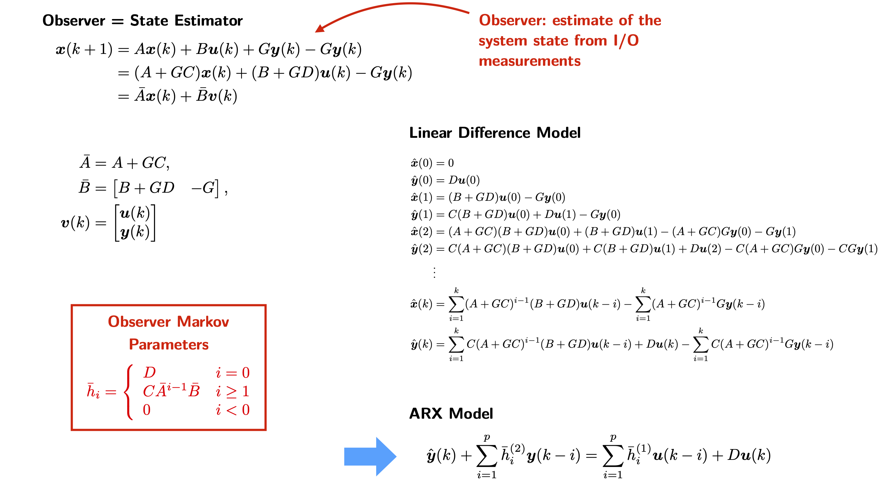
In practice, the primary purpose of introducing an observer is an artifice to compress the data and improve system identification results. A state estimator, also known as an observer, can be used to provide an estimate of the system state from input and output measurements. Add and subtract the term \(G\boldsymbol{y}(k)\) to the right-hand side of the state equation to yield

\begin{align} \boldsymbol{x}(k+1) &= A\boldsymbol{x}(k)+B\boldsymbol{u}(k) + G\boldsymbol{y}(k) - G\boldsymbol{y}(k)\\ &= (A+GC)\boldsymbol{x}(k)+(B+GD)\boldsymbol{u}(k)- G\boldsymbol{y}(k)\\ &= \bar{A}\boldsymbol{x}(k)+\bar{B}\boldsymbol{v}(k) \end{align}

where

\begin{align} \bar{A} &= A+GC,\\ \bar{B} &= \begin{bmatrix} B+GD & -G \end{bmatrix},\\ \boldsymbol{v}(k) &= \begin{bmatrix} \boldsymbol{u}(k)\\ \boldsymbol{y}(k) \end{bmatrix}, \end{align}

and \(G\) is an arbitrary matrix chosen to make the matrix \(\bar{A}\) as stable as desired. The Markov parameters of this observer system are referred as observer Markov parameters. The new input-output in matrix form is therefore

\begin{align} \label{Eq: Observer3} \bar{\boldsymbol{y}} = \bar{\boldsymbol{Y}}\boldsymbol{V} \end{align}

with

\begin{align} \bar{\boldsymbol{y}} &= \begin{bmatrix} \boldsymbol{y}(0) & \boldsymbol{y}(1) & \boldsymbol{y}(2) & \cdots & \boldsymbol{y}(l-1) \end{bmatrix},\\ \bar{\boldsymbol{Y}} &= \begin{bmatrix} D & C\bar{B} & C\bar{A}\bar{B} & \cdots & C\bar{A}^{l-2}\bar{B} \end{bmatrix},\\ \boldsymbol{V} &= \begin{bmatrix} \boldsymbol{u}(0) & \boldsymbol{u}(1) & \boldsymbol{u}(2) & \cdots & \boldsymbol{u}(l-1)\\ &\boldsymbol{v}(0) & \boldsymbol{v}(1) & \cdots & \boldsymbol{v}(l-2)\\ & & \boldsymbol{v}(0) & \cdots & \boldsymbol{v}(l-3)\\ & & & \ddots & \vdots \\ & & & & \boldsymbol{v}(0) \end{bmatrix}. \end{align}

\begin{array}{|c|c|} \hline \# \text{Equations} & \# \text{Unknowns}\\ \hline m\times l & m\times ((r+m)(l-1)+r) \\ \hline \end{array}

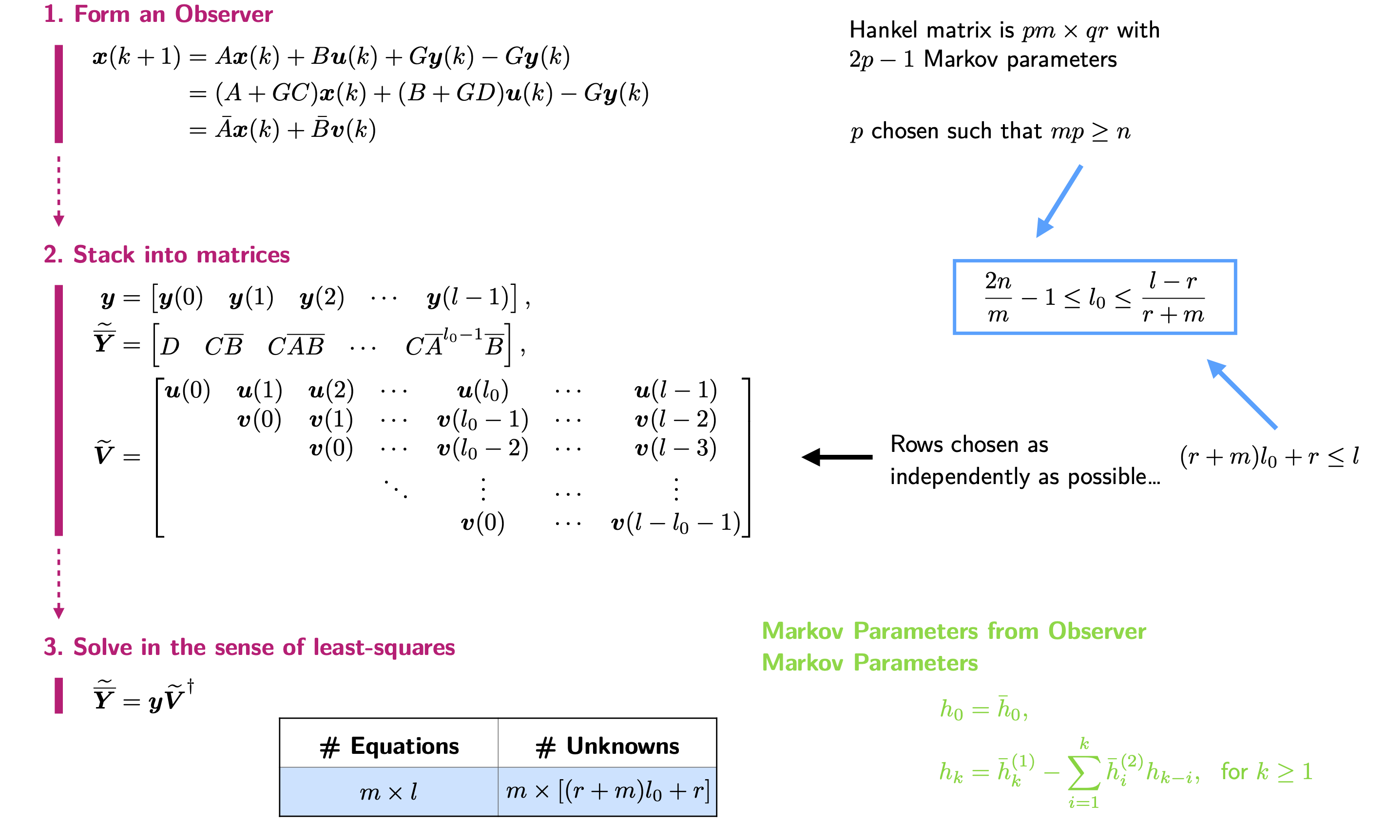
Similarly as before, when \(C\bar{A}^k\bar{B} \simeq 0\) for all time steps \(k\geq l_0\) for some \(l_0\), Eq. (\ref{Eq: Observer3}) can be approximated by

\begin{align} \label{Eq: Observer4} \bar{\boldsymbol{y}} \simeq \widetilde{\bar{\boldsymbol{Y}}}\widetilde{\boldsymbol{V}}, \end{align}

with

\begin{align} \bar{\boldsymbol{y}} &= \begin{bmatrix} \boldsymbol{y}(0) & \boldsymbol{y}(1) & \boldsymbol{y}(2) & \cdots & \boldsymbol{y}(l-1) \end{bmatrix},\\ \widetilde{\bar{\boldsymbol{Y}}} &= \begin{bmatrix} D & C\bar{B} & C\bar{A}\bar{B} & \cdots & C\bar{A}^{l_0-1}\bar{B} \end{bmatrix},\\ \widetilde{\boldsymbol{V}} &= \begin{bmatrix} \boldsymbol{u}(0) & \boldsymbol{u}(1) & \boldsymbol{u}(2) & \cdots & \boldsymbol{u}(l_0) & \cdots & \boldsymbol{u}(l-1)\\ &\boldsymbol{v}(0) & \boldsymbol{v}(1) & \cdots & \boldsymbol{v}(l_0-1) & \cdots & \boldsymbol{v}(l-2)\\ & & \boldsymbol{v}(0) & \cdots & \boldsymbol{v}(l_0-2) & \cdots & \boldsymbol{v}(l-3)\\ & & & \ddots & \vdots & \cdots & \vdots \\ & & & & \boldsymbol{v}(0) & \cdots & \boldsymbol{v}(l-l_0-1) \end{bmatrix}. \end{align}

\begin{array}{|c|c|} \hline \# \text{Equations} & \# \text{Unknowns}\\ \hline m\times l & m\times ((r+m)l_0+r) \\ \hline \end{array}

The first \(l_0+1\) observer Markov parameters approximately satisfy

\begin{align} \widetilde{\bar{\boldsymbol{Y}}} = \bar{\boldsymbol{y}}\widetilde{\boldsymbol{V}}^\dagger, \end{align}

and the approximation error decreases as \(l_0\) increases. To solve for \(\widetilde{\bar{\boldsymbol{Y}}}\) uniquely, all the rows of \(\widetilde{\boldsymbol{V}}\) must be linearly independent. Furthermore, to minimize any numerical error due to the computation of the pseudo-inverse, the rows of \(\widetilde{\boldsymbol{V}}\) should be chosen as independently as possible. As a result, the maximum value of \(l_0\) is the number that maximizes the quantity \((r+m)l_0 + r \leq l\) of independent rows of \(\widetilde{\boldsymbol{V}}\). The maximum \(l_0\) means the upper bound of the order of the deadbeat observer. Furthermore, it is known that the rank of a sufficiently large Hankel matrix \(\boldsymbol{H}_0^{(p, q)}\) is the order of the controllable and observable part of the system (the identified state matrix \(\hat{A}\) represents only the controllable and observable part of the system). The size of the Hankel matrix is \(pm\times qr\) comprised of \(p+q-1\) Markov parameters; with \(p=q\), this means \(2p-1\) Markov parameters. If \(l_0\) is the number of Markov parameters calculated through OKID, it means that \(l_0 = 2p-1\). Assuming \(qr > n\), the maximum rank of \(\boldsymbol{H}_0^{(p, q)}\) is thus \(mp\). If \(p\) is chosen such that \(mp \geq n\), then a realized state matrix \(\hat{A}\) with order \(n\) should exist. Therefore, the number of Markov parameters computed, (l_0\), must be chosen such that

\begin{align} mp \geq n \Leftrightarrow m\dfrac{l_0+1}{2} \geq n, \end{align}

where \(m\) is the number of outputs and \(n\) is the order of the system. To conclude, the lower and upper bounds on \(l_0\) are

\begin{align} \dfrac{2n}{m}-1\leq l_0 \leq \dfrac{l-r}{r+m} \end{align}

with \(l\) being the length of the input signal considered.

The observer Markov parameters can then be used to compute the Markov parameters and the matrices \(A\), \(B\), \(C\) and \(D\).