3.1) Controllability in the discrete-time domain

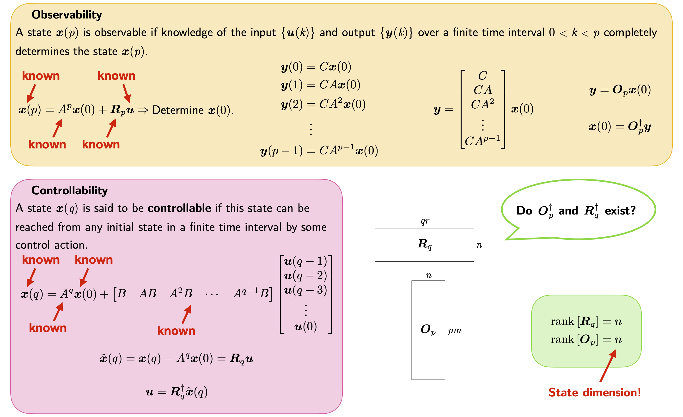
A state \(\boldsymbol{x}(q)\) is said to be controllable or state-controllable if this state can be reached from any initial state of the system in a finite time interval by some control action. If all states are controllable, the system is called completely controllable or simply controllable. Given \(A, B\) and \(\boldsymbol{x}(0)\), the idea is to find the sufficient and necessary condition to determine how to reach \(\boldsymbol{x}(q)\) without ambiguity. It is clear that since \(A\) and \(\boldsymbol{x}(0)\) are given, it is therefore equivalent to determine \(\boldsymbol{x}(q)\) or \(\tilde{\boldsymbol{x}}(q) = \boldsymbol{x}(q) - A^q\boldsymbol{x}(0)\): to determine complete controllability, it is sufficient and necessary to determine whether the zero state (instead of all initial states) can be transferred to all final states.

The solution to the discrete representation at time \(t = q\Delta t\) where \(\Delta t\) is the sampling period is

\begin{align} \boldsymbol{x}(q) = A^q\boldsymbol{x}(0) + \sum_{i=1}^qA^{i-1}B\boldsymbol{u}(q-i) \end{align}

or in a compact matrix form

\begin{align} \boldsymbol{x}(q) = A^q\boldsymbol{x}(0) + \begin{bmatrix} B & AB & A^2B & \cdots & A^{q-1}B \end{bmatrix} \begin{bmatrix} \boldsymbol{u}(q-1)\\ \boldsymbol{u}(q-2)\\ \boldsymbol{u}(q-3)\\ \vdots\\ \boldsymbol{u}(0) \end{bmatrix}. \end{align}

The expression of \(\tilde{\boldsymbol{x}}(q)\) can be written as

\begin{align} \label{Eq: x_tilde(q)} \tilde{\boldsymbol{x}}(q) = \boldsymbol{R}^{(q)} \overline{\boldsymbol{u}} \end{align}

where

\begin{align} \label{Eq: Rq} \boldsymbol{R}^{(q)} = \begin{bmatrix} B & AB & A^2B & \cdots & A^{q-1}B \end{bmatrix}, \end{align}

and

\begin{align} \overline{\boldsymbol{u}} = \begin{bmatrix} \boldsymbol{u}(q-1)\\ \boldsymbol{u}(q-2)\\ \boldsymbol{u}(q-3)\\ \vdots\\ \boldsymbol{u}(0) \end{bmatrix}. \end{align}

\(\boldsymbol{R}^{(q)}\) is called the controllability matrix. Reaching \(\boldsymbol{x}(q)\) without ambiguity is thus equivalent to find a solution of Eq. (\ref{Eq: x_tilde(q)}) for \(\overline{\boldsymbol{u}}\). Therefore, a discrete time-invariant linear system of order \(n\) is controllable if and only if the \(n\times qr\) block controllability matrix \(\boldsymbol{R}^{(q)}\) has rank \(n\) (assuming \(qr > n\)).

3.2) Observability in the discrete-time domain

A state \(\boldsymbol{x}(p)\) is observable if the knowledge of the input \(\boldsymbol{u}(k)\) and output \(\boldsymbol{y}(k)\) over a finite time interval \(0\leq k\leq p-1\) completely determines the state \(\boldsymbol{x}(p)\):

\begin{align} \boldsymbol{x}(p) = A^p\boldsymbol{x}(0) + \sum_{i=1}^pA^{i-1}B\boldsymbol{u}(p-i). \end{align}

With knowledge of the system matrices \(A\) and \(B\) and the control input \(\boldsymbol{u}(k)\), \(0\leq k\leq p-1\), it is necessary and sufficient to see whether the initial state \(\boldsymbol{x}(0)\) can be completely determined from the output sequence \(\boldsymbol{y}(k)\), \(0\leq k\leq p-1\). In a compact matrix form, we can write

\begin{align} \overline{\boldsymbol{y}} = \begin{bmatrix} \boldsymbol{y}(0)\\ \boldsymbol{y}(1)\\ \boldsymbol{y}(2)\\ \vdots\\ \boldsymbol{y}(p-1) \end{bmatrix} = \begin{bmatrix} C\\ CA\\ CA^2\\ \vdots\\ CA^{p-1} \end{bmatrix}\boldsymbol{x}(0) = \boldsymbol{O}^{(p)}\boldsymbol{x}(0), \end{align}

where a unique solution for \(\boldsymbol{x}(0)\) exists if and only if \(\boldsymbol{O}^{(p)}\) has rank \(n\) (full rank, assuming \(pm > n\)). Thus, a discrete time-invariant linear system of order \(n\) is observable if and only if the \(pm\times n\) block observability matrix \(\boldsymbol{O}^{(p)}\) has rank \(n\), where

\begin{align} \label{Eq: Op} \boldsymbol{O}^{(p)} = \begin{bmatrix} C\\ CA\\ CA^2\\ \vdots\\ CA^{p-1} \end{bmatrix}. \end{align}

These two notions of controllability and observability will be of central attention in chapter 5 for the development of the Eigensystem Realization Algorithm.

3.3) Summary