2.1) Continuous-Time State-Space Models

The equations of motion for a finite-dimensional linear-dynamic system are a set of \(n\) first-order differential equations \eqref{Eq: continuous time-invariant linear system x_dot} along with an initial condition \(\boldsymbol{x}(t_0)\). The \(n\)-dimensional state \(\boldsymbol{x}(t)\) is most often related to the output through the measurement equation \eqref{Eq: continuous time-invariant linear system y}.

\begin{align} \label{Eq: continuous time-invariant linear system x_dot} \dot{\boldsymbol{x}}(t) &= A_c\boldsymbol{x}(t)+B_c\boldsymbol{u}(t)\\ \label{Eq: continuous time-invariant linear system y} \boldsymbol{y}(t) &= C\boldsymbol{x}(t)+D\boldsymbol{u}(t). \end{align}

This system of equations constitutes a continuous-time state-space model of a dynamical system. Given the initial condition \(\boldsymbol{x}(t_0)\) at some \(t=t_0\), solving for \(\boldsymbol{x}(t)\) for \(t>t_0\) yields

\begin{align} \boldsymbol{x}(t) = e^{A_c(t-t_0)}\boldsymbol{x}(t_0)+\int_{t_0}^te^{A_c(t-\tau)}B_c\boldsymbol{u}(\tau)\mathrm{d}\tau. \end{align}

Without loss of generality, we will consider that \(t_0 = 0\).

2.2) Discrete-Time State-Space Models

Dynamic systems are typically modeled by continuous-time or discrete-time equations. A close approximation of a continuous-time model can be obtained by a discrete one provided that the sampling rate is sufficiently high. A linear discrete system is most commonly described by an \(n^{\text{th}}\) order difference equation, the weighting sequence, or a discrete state-space model. Let \(\Delta t\) be a constant time interval and \(f=1/\Delta t\) the sampling rate. Continuous versions of the \(A\) and \(B\) matrices are

\begin{align} \label{Eq: A Discrete_time} A &= e^{A_c\Delta t},\\ \label{Eq: B Discrete_time} B &= \int_0^{\Delta t}e^{A_c\tau}\mathrm{d}\tau B_c,\\ \boldsymbol{x}(k+1) &= \boldsymbol{x}((k+1)\Delta t),\\ \boldsymbol{u}(k) &= \boldsymbol{u}(k\Delta t). \end{align}

The discrete-time matrices \(A\) and \(B\) in \eqref{Eq: A Discrete_time} and \eqref{Eq: B Discrete_time} may be computed by the following series expansions:

\begin{align} \label{Eq: A series} A &= e^{A_c\Delta t} = \sum_{i=0}^{\infty}\dfrac{1}{i!}\left[A_c\Delta t\right]^i,\\ \label{Eq: B series} B &= \int_0^{\Delta t}e^{A_c\tau}\mathrm{d}\tau B_c = \left[\sum_{i=0}^{\infty}\dfrac{1}{i!}A_c^i\left(\Delta t\right)^{i+1}\right]B_c. \end{align}

A sufficient condition for these series expansions to converge is that the continuous-time state matrix \(A_c\) is asymptotically stable in the sense that the real parts of all its eigenvalues are negative. If none of the eigenvalues of \(A_c\) are zero, the discrete-time matrix \(B\) may also be computed by

\begin{align} B = \left[A-I\right]A_c^{-1}B_c. \end{align}

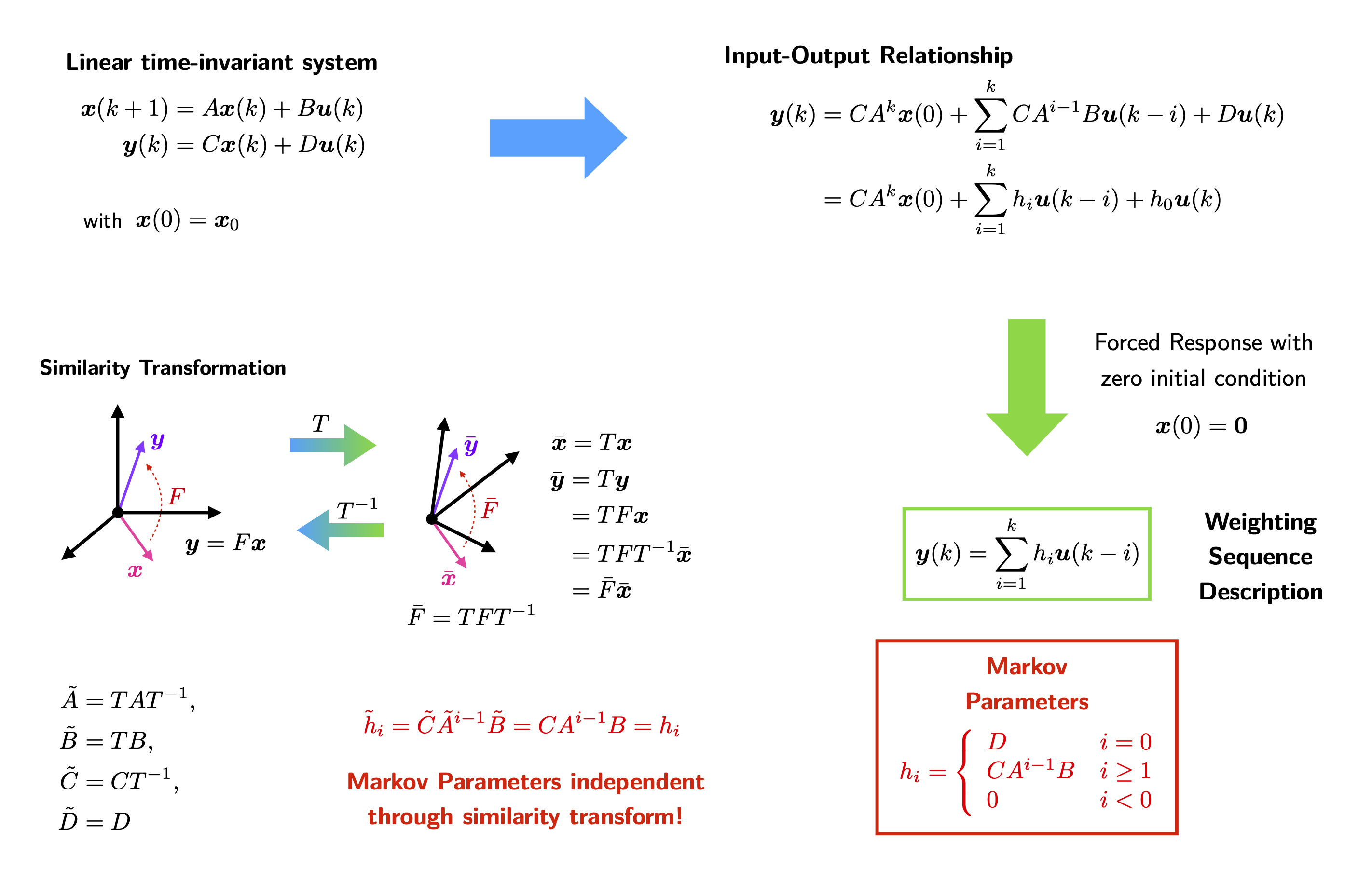
Therefore, a discrete-time invariant linear system can be represented by

\begin{align} \label{Eq: discrete time-invariant linear system x(k+1)} \boldsymbol{x}(k+1) &= A\boldsymbol{x}(k)+B\boldsymbol{u}(k)\\ \boldsymbol{y}(k) &= C\boldsymbol{x}(k)+D\boldsymbol{u}(k) \end{align}

together with an initial state vector \(\boldsymbol{x}(0)\), where \(\boldsymbol{x}\), \(\boldsymbol{u}\) and \(\boldsymbol{y}\) are the state, control input and output vectors respectively. The constant matrices \(A\), \(B\), \(C\) and \(D\) with appropriate dimensions represent the internal operation of the linear system, and are used to determine the system's response to any input.

2.3) Weighting Sequence Description and Markov Parameters

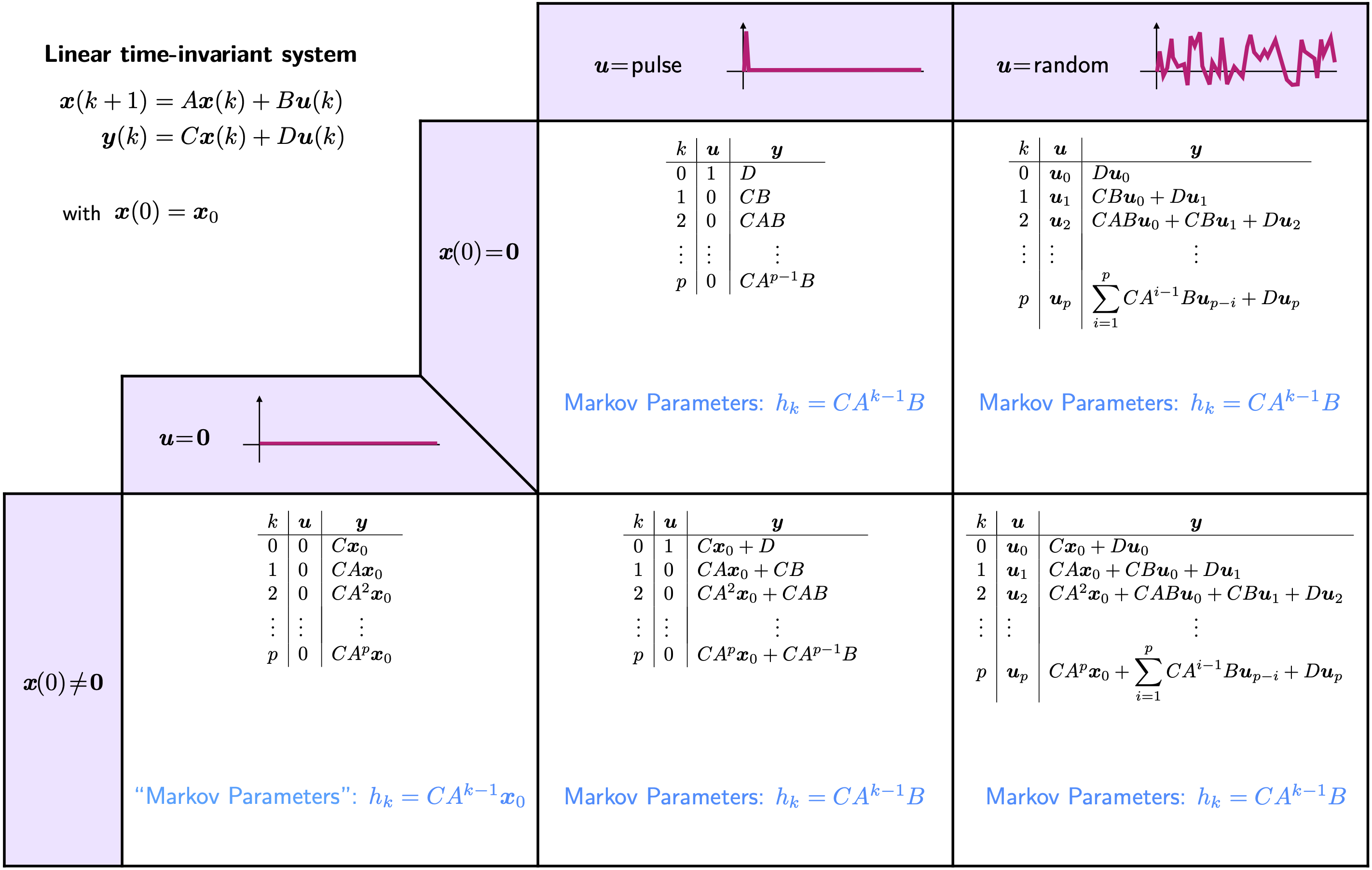
Solving for the state \(\boldsymbol{x}(k)\) and the output \(\boldsymbol{y}(k)\) with arbitrary initial condition \(\boldsymbol{x}(0)\) in terms of the previous inputs \(\boldsymbol{u}(i)\), \(i=0, 1, \ldots, k\), yields

\begin{align} \boldsymbol{x}(k) &= A^k\boldsymbol{x}(0) + \sum_{i=1}^kA^{i-1}B\boldsymbol{u}(k-i),\\ \boldsymbol{y}(k) &= CA^k\boldsymbol{x}(0) + \sum_{i=1}^kCA^{i-1}B\boldsymbol{u}(k-i) + D\boldsymbol{u}(k). \end{align}

It appears naturally that the constant matrices sequence

\begin{align} \begin{split} h_0 &= D,\\ h_1 &= CB,\\ h_2 &= CAB, \\ & \hspace{0.5em} \vdots \\ h_k &= CA^{k-1}B,\\ & \hspace{0.5em} \vdots \end{split} \end{align}

plays an important role in identifying a mathematical model for linear dynamical systems. In fact, with zero initial condition \(\boldsymbol{x}(0)=\boldsymbol{0}\), considering the response to a pulse sequence such that for \(j=1, 2, \ldots, r\),

\begin{align} u_j(i) = \left\lbrace\begin{array}{ll} 1 & \text{for } i = 0\\ 0 & \text{for } i = 1, 2, \ldots \end{array}\right. \end{align}

the \(r\) corresponding outputs \(\left\lbrace\boldsymbol{y}^{(j)}(i)\right\rbrace_{i=1, 2, \ldots}\) can be assembled at each time step to recover the sequence \(\left\lbrace h_i\right\rbrace_{i=1, 2, \ldots}\) as follows:

\begin{align} h_i = \begin{bmatrix} \boldsymbol{y}^{(1)}(i) & \boldsymbol{y}^{(2)}(i) & \cdots & \boldsymbol{y}^{(r)}(i) \end{bmatrix}. \end{align}

The constant matrices in the sequence \(\left\lbrace h_i\right\rbrace_{i=1, 2, \ldots}\) are known as system Markov parameters or, in short, Markov parameters. It is obvious that the matrices \(A, B, C, D\) are embedded in the Markov parameter sequence; undeniably, the determination of Markov parameters should be tantamount to system identification. The general form of the Markov parameters is thus

\begin{align} \label{Eq: Markov parameters} h_{i} = \left\lbrace\begin{array}{ll} D & i = 0,\\ CA^{i-1}B & i \geq 1,\\ 0 & i < 0. \end{array}\right. \end{align}

2.4) Summary